
PySpark is a python wrapper built around Spark – a unified Data Science and Analysis framework for working with Big Data. It combines the benefits and functions we can achieve when working with data whilst using popular libraries such as Pandas, Scikit-Learn ,SQL,etc.
PySpark is the Python API for Spark.
It offers all of these features in one library or framework to make our work easier. Hence you can do all your data science and Big Data Analysis all in one unified framework – from data preparation to model building to deployment.
PySpark works around 2 main key data structures which include:
- RDD : Resilient Distributed Datasets – which is the legacy API and is fault tolerant
- DataFrame: this is the current API which is similary to Dataframe concepts in Pandas or R.
So why use PySpark? PySpark is useful when working with Big Data especially datasets that are too huge to fit on one machine when analysing them. Hence with PySpark you can analyze huge datasets using a distributed service of systems.
However you can also use PySpark on a single local machine.
By the end of this tutorial we will learn
- What PySpark is
- How to Install PySpark
- Working with Datasets using PySpark
- Machine Learning with PySpark
- etc
What is PySpark?
Pyspark is Python Wrapper around Spark – unified framework for analyzing Big Data. Hence the name Py- Spark. It combines the best of Spark with the convenience of Python since python has now become the defacto language for Programming Languages.
How to Install PySpark
There are several ways we can install pyspark on your system. These methods include
- Using Virtual Environment (recommended for this tutorial)
- Using Docker
- Using DataBricks
- Local Installation
The simpliest way is to install pyspark inside a virtual environment. You can use any virtualenv package you want but in our case we will be using Pipenv. To install pipenv you can do
pip install pipenv
You can then set up your pyspark workspace via
mkdir myworkspace
cd myworkspace
pipenv install pyspark jupyterlab matplotlib scikit-learn
Since we will be working inside jupyter notebook or jupyter lab we will install it alongside. You can now spin up your workspace by this command
pipenv shell
pipenv run jupyter lab
You can also use docker and pull the docker image for pyspark built by the jupyter team.
docker pull jupyter/pyspark-notebook
Data Analysis with PySpark – Working with Datasets
In this section we will be analyzing a simple dataset using PySpark. The advantages of pyspark is that it gives you the option of a UI in which you can visualize what is going behind the scene and how actions and transformations are done.
Let us first create a Spark Session or A Spark Context which is the main entry point for all our analysis.
# Create A SparkSession
from pyspark.sql import SparkSession
spark = SparkSession.builder.appName("PySparkTut").getOrCreate()
You can get the UI via typing either the spark variable created or the spark context variable created
# Load PySPark
from pyspark import SparkContext
sc = SparkContext(master="local[2]")
# Using Spark UI
sc
Out[3]:
SparkContext
Version v3.0.1
Master local[2]
AppName pyspark-shell
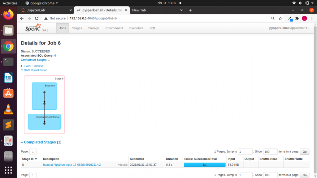
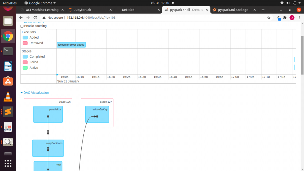
Clicking on the Spark UI will open a UI on the port given like below that shows the jobs and stages of each action and transformation in pyspark.
Working with CSV Datasets
# Read A DataSet without header
df = spark.read.csv('diamonds.csv')
In [13]:
# Preview dataset
df.show()
+-----+---------+-----+-------+-----+-----+-----+----+----+----+
|  _c0|      _c1|  _c2|    _c3|  _c4|  _c5|  _c6| _c7| _c8| _c9|
+-----+---------+-----+-------+-----+-----+-----+----+----+----+
|carat|      cut|color|clarity|depth|table|price|   x|   y|   z|
| 0.23|    Ideal|    E|    SI2| 61.5|   55|  326|3.95|3.98|2.43|
| 0.21|  Premium|    E|    SI1| 59.8|   61|  326|3.89|3.84|2.31|
| 0.23|     Good|    E|    VS1| 56.9|   65|  327|4.05|4.07|2.31|
| 0.29|  Premium|    I|    VS2| 62.4|   58|  334| 4.2|4.23|2.63|
| 0.31|     Good|    J|    SI2| 63.3|   58|  335|4.34|4.35|2.75|
| 0.24|Very Good|    J|   VVS2| 62.8|   57|  336|3.94|3.96|2.48|
| 0.24|Very Good|    I|   VVS1| 62.3|   57|  336|3.95|3.98|2.47|
| 0.26|Very Good|    H|    SI1| 61.9|   55|  337|4.07|4.11|2.53|
| 0.22|     Fair|    E|    VS2| 65.1|   61|  337|3.87|3.78|2.49|
| 0.23|Very Good|    H|    VS1| 59.4|   61|  338|   4|4.05|2.39|
|  0.3|     Good|    J|    SI1|   64|   55|  339|4.25|4.28|2.73|
| 0.23|    Ideal|    J|    VS1| 62.8|   56|  340|3.93| 3.9|2.46|
| 0.22|  Premium|    F|    SI1| 60.4|   61|  342|3.88|3.84|2.33|
| 0.31|    Ideal|    J|    SI2| 62.2|   54|  344|4.35|4.37|2.71|
|  0.2|  Premium|    E|    SI2| 60.2|   62|  345|3.79|3.75|2.27|
| 0.32|  Premium|    E|     I1| 60.9|   58|  345|4.38|4.42|2.68|
|  0.3|    Ideal|    I|    SI2|   62|   54|  348|4.31|4.34|2.68|
|  0.3|     Good|    J|    SI1| 63.4|   54|  351|4.23|4.29| 2.7|
|  0.3|     Good|    J|    SI1| 63.8|   56|  351|4.23|4.26|2.71|
+-----+---------+-----+-------+-----+-----+-----+----+----+----+
only showing top 20 rows
In [62]:
# Read A DataSet with header/column names
df = spark.read.csv('diamonds.csv',header=True)
In [15]:
df.show()
+-----+---------+-----+-------+-----+-----+-----+----+----+----+
|carat|      cut|color|clarity|depth|table|price|   x|   y|   z|
+-----+---------+-----+-------+-----+-----+-----+----+----+----+
| 0.23|    Ideal|    E|    SI2| 61.5|   55|  326|3.95|3.98|2.43|
| 0.21|  Premium|    E|    SI1| 59.8|   61|  326|3.89|3.84|2.31|
| 0.23|     Good|    E|    VS1| 56.9|   65|  327|4.05|4.07|2.31|
| 0.29|  Premium|    I|    VS2| 62.4|   58|  334| 4.2|4.23|2.63|
| 0.31|     Good|    J|    SI2| 63.3|   58|  335|4.34|4.35|2.75|
| 0.24|Very Good|    J|   VVS2| 62.8|   57|  336|3.94|3.96|2.48|
| 0.24|Very Good|    I|   VVS1| 62.3|   57|  336|3.95|3.98|2.47|
| 0.26|Very Good|    H|    SI1| 61.9|   55|  337|4.07|4.11|2.53|
| 0.22|     Fair|    E|    VS2| 65.1|   61|  337|3.87|3.78|2.49|
| 0.23|Very Good|    H|    VS1| 59.4|   61|  338|   4|4.05|2.39|
|  0.3|     Good|    J|    SI1|   64|   55|  339|4.25|4.28|2.73|
| 0.23|    Ideal|    J|    VS1| 62.8|   56|  340|3.93| 3.9|2.46|
| 0.22|  Premium|    F|    SI1| 60.4|   61|  342|3.88|3.84|2.33|
| 0.31|    Ideal|    J|    SI2| 62.2|   54|  344|4.35|4.37|2.71|
|  0.2|  Premium|    E|    SI2| 60.2|   62|  345|3.79|3.75|2.27|
| 0.32|  Premium|    E|     I1| 60.9|   58|  345|4.38|4.42|2.68|
|  0.3|    Ideal|    I|    SI2|   62|   54|  348|4.31|4.34|2.68|
|  0.3|     Good|    J|    SI1| 63.4|   54|  351|4.23|4.29| 2.7|
|  0.3|     Good|    J|    SI1| 63.8|   56|  351|4.23|4.26|2.71|
|  0.3|Very Good|    J|    SI1| 62.7|   59|  351|4.21|4.27|2.66|
+-----+---------+-----+-------+-----+-----+-----+----+----+----+
only showing top 20 rows
In [16]:
# Columns
df.columns
Out[16]:
['carat', 'cut', 'color', 'clarity', 'depth', 'table', 'price', 'x', 'y', 'z']
In [20]:
# Shape (rows + columns)
(df.count() ,len(df.columns))
Out[20]:
(53940, 10)
In [21]:
# Number of columns
len(df.columns)
Out[21]:
10
In [22]:
# Number of rows
df.count()
Out[22]:
53940
In [24]:
# Descriptive Analysis
df.describe().show()
+-------+------------------+---------+-----+-------+------------------+------------------+-----------------+------------------+------------------+------------------+
|summary|             carat|      cut|color|clarity|             depth|             table|            price|                 x|                 y|                 z|
+-------+------------------+---------+-----+-------+------------------+------------------+-----------------+------------------+------------------+------------------+
|  count|             53940|    53940|53940|  53940|             53940|             53940|            53940|             53940|             53940|             53940|
|   mean|0.7979397478679852|     null| null|   null| 61.74940489432624| 57.45718390804603|3932.799721913237| 5.731157211716609| 5.734525954764462|3.5387337782723316|
| stddev|0.4740112444054196|     null| null|   null|1.4326213188336525|2.2344905628213247|3989.439738146397|1.1217607467924915|1.1421346741235616|0.7056988469499883|
|    min|               0.2|     Fair|    D|     I1|                43|                43|             1000|                 0|                 0|                 0|
|    max|              5.01|Very Good|    J|   VVS2|                79|                95|             9999|              9.86|              9.94|              8.06|
+-------+------------------+---------+-----+-------+------------------+------------------+-----------------+------------------+------------------+------------------+
In [25]:
# Pick a column & Get summary/describe a selected column
df.describe('carat').show()
+-------+------------------+
|summary|             carat|
+-------+------------------+
|  count|             53940|
|   mean|0.7979397478679852|
| stddev|0.4740112444054196|
|    min|               0.2|
|    max|              5.01|
+-------+------------------+
In [26]:
# Preview the First Row
df.first()
Out[26]:
Row(carat='0.23', cut='Ideal', color='E', clarity='SI2', depth='61.5', table='55', price='326', x='3.95', y='3.98', z='2.43')
In [31]:
# Preview the first 10 rows
# Like a list
df.head(10)
Out[31]:
[Row(carat='0.23', cut='Ideal', color='E', clarity='SI2', depth='61.5', table='55', price='326', x='3.95', y='3.98', z='2.43'),
 Row(carat='0.21', cut='Premium', color='E', clarity='SI1', depth='59.8', table='61', price='326', x='3.89', y='3.84', z='2.31'),
 Row(carat='0.23', cut='Good', color='E', clarity='VS1', depth='56.9', table='65', price='327', x='4.05', y='4.07', z='2.31'),
 Row(carat='0.29', cut='Premium', color='I', clarity='VS2', depth='62.4', table='58', price='334', x='4.2', y='4.23', z='2.63'),
 Row(carat='0.31', cut='Good', color='J', clarity='SI2', depth='63.3', table='58', price='335', x='4.34', y='4.35', z='2.75'),
 Row(carat='0.24', cut='Very Good', color='J', clarity='VVS2', depth='62.8', table='57', price='336', x='3.94', y='3.96', z='2.48'),
 Row(carat='0.24', cut='Very Good', color='I', clarity='VVS1', depth='62.3', table='57', price='336', x='3.95', y='3.98', z='2.47'),
 Row(carat='0.26', cut='Very Good', color='H', clarity='SI1', depth='61.9', table='55', price='337', x='4.07', y='4.11', z='2.53'),
 Row(carat='0.22', cut='Fair', color='E', clarity='VS2', depth='65.1', table='61', price='337', x='3.87', y='3.78', z='2.49'),
 Row(carat='0.23', cut='Very Good', color='H', clarity='VS1', depth='59.4', table='61', price='338', x='4', y='4.05', z='2.39')]
In [32]:
# Method 2: Useful Action with show()
# Show first 10 datapoints
df.show(10)
+-----+---------+-----+-------+-----+-----+-----+----+----+----+
|carat|      cut|color|clarity|depth|table|price|   x|   y|   z|
+-----+---------+-----+-------+-----+-----+-----+----+----+----+
| 0.23|    Ideal|    E|    SI2| 61.5|   55|  326|3.95|3.98|2.43|
| 0.21|  Premium|    E|    SI1| 59.8|   61|  326|3.89|3.84|2.31|
| 0.23|     Good|    E|    VS1| 56.9|   65|  327|4.05|4.07|2.31|
| 0.29|  Premium|    I|    VS2| 62.4|   58|  334| 4.2|4.23|2.63|
| 0.31|     Good|    J|    SI2| 63.3|   58|  335|4.34|4.35|2.75|
| 0.24|Very Good|    J|   VVS2| 62.8|   57|  336|3.94|3.96|2.48|
| 0.24|Very Good|    I|   VVS1| 62.3|   57|  336|3.95|3.98|2.47|
| 0.26|Very Good|    H|    SI1| 61.9|   55|  337|4.07|4.11|2.53|
| 0.22|     Fair|    E|    VS2| 65.1|   61|  337|3.87|3.78|2.49|
| 0.23|Very Good|    H|    VS1| 59.4|   61|  338|   4|4.05|2.39|
+-----+---------+-----+-------+-----+-----+-----+----+----+----+
only showing top 10 rows
In [33]:
# Get Last Rows
df.tail(5)
Out[33]:
[Row(carat='0.72', cut='Ideal', color='D', clarity='SI1', depth='60.8', table='57', price='2757', x='5.75', y='5.76', z='3.5'),
 Row(carat='0.72', cut='Good', color='D', clarity='SI1', depth='63.1', table='55', price='2757', x='5.69', y='5.75', z='3.61'),
 Row(carat='0.7', cut='Very Good', color='D', clarity='SI1', depth='62.8', table='60', price='2757', x='5.66', y='5.68', z='3.56'),
 Row(carat='0.86', cut='Premium', color='H', clarity='SI2', depth='61', table='58', price='2757', x='6.15', y='6.12', z='3.74'),
 Row(carat='0.75', cut='Ideal', color='D', clarity='SI2', depth='62.2', table='55', price='2757', x='5.83', y='5.87', z='3.64')]
Selection of columns
- .select ###### Note
- Dot & Bracket Notation only gives the column name not the entire column
- [‘colA’]*
- .colA*
In [35]:
# List all Columns
df.columns
Out[35]:
['carat', 'cut', 'color', 'clarity', 'depth', 'table', 'price', 'x', 'y', 'z']
In [37]:
# Select A Column
df.select('carat').show()
+-----+
|carat|
+-----+
| 0.23|
| 0.21|
| 0.23|
| 0.29|
| 0.31|
| 0.24|
| 0.24|
| 0.26|
| 0.22|
| 0.23|
|  0.3|
| 0.23|
| 0.22|
| 0.31|
|  0.2|
| 0.32|
|  0.3|
|  0.3|
|  0.3|
|  0.3|
+-----+
only showing top 20 rows
In [40]:
# Select A Column irrespective of column word case
# will work irrespective of the case of the column once it is found within the dataset
df.select('CARAT').show()
+-----+
|CARAT|
+-----+
| 0.23|
| 0.21|
| 0.23|
| 0.29|
| 0.31|
| 0.24|
| 0.24|
| 0.26|
| 0.22|
| 0.23|
|  0.3|
| 0.23|
| 0.22|
| 0.31|
|  0.2|
| 0.32|
|  0.3|
|  0.3|
|  0.3|
|  0.3|
+-----+
only showing top 20 rows
In [41]:
# This is not as we would expect in pandas
# For Bracket Notation : pick column name not the entire columne
df['carat']
Out[41]:
Column<b'carat'>
In [44]:
# This is not as we would expect in pandas
# For Dot Notation : pick column name not the entire column
df.carat
Out[44]:
Column<b'carat'>
In [45]:
# Select Multiple Columns
df.select('carat','cut').show(5)
+-----+-------+
|carat|    cut|
+-----+-------+
| 0.23|  Ideal|
| 0.21|Premium|
| 0.23|   Good|
| 0.29|Premium|
| 0.31|   Good|
+-----+-------+
only showing top 5 rows
Column Filtering and Applying Conditions
With PySpark you can also filter your dataset per conditionand also apply conditions .
- .filter
- .where
In [46]:
# Filter of Columns
# Apply A Condition
df.show(10)
+-----+---------+-----+-------+-----+-----+-----+----+----+----+
|carat|      cut|color|clarity|depth|table|price|   x|   y|   z|
+-----+---------+-----+-------+-----+-----+-----+----+----+----+
| 0.23|    Ideal|    E|    SI2| 61.5|   55|  326|3.95|3.98|2.43|
| 0.21|  Premium|    E|    SI1| 59.8|   61|  326|3.89|3.84|2.31|
| 0.23|     Good|    E|    VS1| 56.9|   65|  327|4.05|4.07|2.31|
| 0.29|  Premium|    I|    VS2| 62.4|   58|  334| 4.2|4.23|2.63|
| 0.31|     Good|    J|    SI2| 63.3|   58|  335|4.34|4.35|2.75|
| 0.24|Very Good|    J|   VVS2| 62.8|   57|  336|3.94|3.96|2.48|
| 0.24|Very Good|    I|   VVS1| 62.3|   57|  336|3.95|3.98|2.47|
| 0.26|Very Good|    H|    SI1| 61.9|   55|  337|4.07|4.11|2.53|
| 0.22|     Fair|    E|    VS2| 65.1|   61|  337|3.87|3.78|2.49|
| 0.23|Very Good|    H|    VS1| 59.4|   61|  338|   4|4.05|2.39|
+-----+---------+-----+-------+-----+-----+-----+----+----+----+
only showing top 10 rows
In [47]:
# Method 1:using filter
df.filter(df['cut'] == "Good").show()
+-----+----+-----+-------+-----+-----+-----+----+----+----+
|carat| cut|color|clarity|depth|table|price|   x|   y|   z|
+-----+----+-----+-------+-----+-----+-----+----+----+----+
| 0.23|Good|    E|    VS1| 56.9|   65|  327|4.05|4.07|2.31|
| 0.31|Good|    J|    SI2| 63.3|   58|  335|4.34|4.35|2.75|
|  0.3|Good|    J|    SI1|   64|   55|  339|4.25|4.28|2.73|
|  0.3|Good|    J|    SI1| 63.4|   54|  351|4.23|4.29| 2.7|
|  0.3|Good|    J|    SI1| 63.8|   56|  351|4.23|4.26|2.71|
|  0.3|Good|    I|    SI2| 63.3|   56|  351|4.26| 4.3|2.71|
| 0.23|Good|    F|    VS1| 58.2|   59|  402|4.06|4.08|2.37|
| 0.23|Good|    E|    VS1| 64.1|   59|  402|3.83|3.85|2.46|
| 0.31|Good|    H|    SI1|   64|   54|  402|4.29|4.31|2.75|
| 0.26|Good|    D|    VS2| 65.2|   56|  403|3.99|4.02|2.61|
| 0.26|Good|    D|    VS1| 58.4|   63|  403|4.19|4.24|2.46|
| 0.32|Good|    H|    SI2| 63.1|   56|  403|4.34|4.37|2.75|
| 0.32|Good|    H|    SI2| 63.8|   56|  403|4.36|4.38|2.79|
|  0.3|Good|    I|    SI1| 63.2|   55|  405|4.25|4.29| 2.7|
|  0.3|Good|    H|    SI1| 63.7|   57|  554|4.28|4.26|2.72|
| 0.26|Good|    E|   VVS1| 57.9|   60|  554|4.22|4.25|2.45|
|  0.7|Good|    E|    VS2| 57.5|   58| 2759|5.85| 5.9|3.38|
|  0.7|Good|    F|    VS1| 59.4|   62| 2759|5.71|5.76| 3.4|
|  0.7|Good|    H|   VVS2| 62.1|   64| 2767|5.62|5.65| 3.5|
| 0.71|Good|    E|    VS2| 59.2|   61| 2772| 5.8|5.88|3.46|
+-----+----+-----+-------+-----+-----+-----+----+----+----+
only showing top 20 rows
In [48]:
# Method 1:using filter
df.filter(df.carat >= 0.7).show()
+-----+---------+-----+-------+-----+-----+-----+----+----+----+
|carat|      cut|color|clarity|depth|table|price|   x|   y|   z|
+-----+---------+-----+-------+-----+-----+-----+----+----+----+
|  0.7|    Ideal|    E|    SI1| 62.5|   57| 2757| 5.7|5.72|3.57|
| 0.86|     Fair|    E|    SI2| 55.1|   69| 2757|6.45|6.33|3.52|
|  0.7|    Ideal|    G|    VS2| 61.6|   56| 2757| 5.7|5.67| 3.5|
| 0.71|Very Good|    E|    VS2| 62.4|   57| 2759|5.68|5.73|3.56|
| 0.78|Very Good|    G|    SI2| 63.8|   56| 2759|5.81|5.85|3.72|
|  0.7|     Good|    E|    VS2| 57.5|   58| 2759|5.85| 5.9|3.38|
|  0.7|     Good|    F|    VS1| 59.4|   62| 2759|5.71|5.76| 3.4|
| 0.96|     Fair|    F|    SI2| 66.3|   62| 2759|6.27|5.95|4.07|
| 0.73|Very Good|    E|    SI1| 61.6|   59| 2760|5.77|5.78|3.56|
|  0.8|  Premium|    H|    SI1| 61.5|   58| 2760|5.97|5.93|3.66|
| 0.75|Very Good|    D|    SI1| 63.2|   56| 2760| 5.8|5.75|3.65|
| 0.75|  Premium|    E|    SI1| 59.9|   54| 2760|   6|5.96|3.58|
| 0.74|    Ideal|    G|    SI1| 61.6|   55| 2760| 5.8|5.85|3.59|
| 0.75|  Premium|    G|    VS2| 61.7|   58| 2760|5.85|5.79|3.59|
|  0.8|    Ideal|    I|    VS1| 62.9|   56| 2760|5.94|5.87|3.72|
| 0.75|    Ideal|    G|    SI1| 62.2|   55| 2760|5.87| 5.8|3.63|
|  0.8|  Premium|    G|    SI1|   63|   59| 2760| 5.9|5.81|3.69|
| 0.74|    Ideal|    I|   VVS2| 62.3|   55| 2761|5.77|5.81|3.61|
| 0.81|    Ideal|    F|    SI2| 58.8|   57| 2761|6.14|6.11| 3.6|
|  0.8|    Ideal|    F|    SI2| 61.4|   57| 2761|5.96|   6|3.67|
+-----+---------+-----+-------+-----+-----+-----+----+----+----+
only showing top 20 rows
In [49]:
# Method 2: where
df.where(df['cut'] == 'Good').show()
+-----+----+-----+-------+-----+-----+-----+----+----+----+
|carat| cut|color|clarity|depth|table|price|   x|   y|   z|
+-----+----+-----+-------+-----+-----+-----+----+----+----+
| 0.23|Good|    E|    VS1| 56.9|   65|  327|4.05|4.07|2.31|
| 0.31|Good|    J|    SI2| 63.3|   58|  335|4.34|4.35|2.75|
|  0.3|Good|    J|    SI1|   64|   55|  339|4.25|4.28|2.73|
|  0.3|Good|    J|    SI1| 63.4|   54|  351|4.23|4.29| 2.7|
|  0.3|Good|    J|    SI1| 63.8|   56|  351|4.23|4.26|2.71|
|  0.3|Good|    I|    SI2| 63.3|   56|  351|4.26| 4.3|2.71|
| 0.23|Good|    F|    VS1| 58.2|   59|  402|4.06|4.08|2.37|
| 0.23|Good|    E|    VS1| 64.1|   59|  402|3.83|3.85|2.46|
| 0.31|Good|    H|    SI1|   64|   54|  402|4.29|4.31|2.75|
| 0.26|Good|    D|    VS2| 65.2|   56|  403|3.99|4.02|2.61|
| 0.26|Good|    D|    VS1| 58.4|   63|  403|4.19|4.24|2.46|
| 0.32|Good|    H|    SI2| 63.1|   56|  403|4.34|4.37|2.75|
| 0.32|Good|    H|    SI2| 63.8|   56|  403|4.36|4.38|2.79|
|  0.3|Good|    I|    SI1| 63.2|   55|  405|4.25|4.29| 2.7|
|  0.3|Good|    H|    SI1| 63.7|   57|  554|4.28|4.26|2.72|
| 0.26|Good|    E|   VVS1| 57.9|   60|  554|4.22|4.25|2.45|
|  0.7|Good|    E|    VS2| 57.5|   58| 2759|5.85| 5.9|3.38|
|  0.7|Good|    F|    VS1| 59.4|   62| 2759|5.71|5.76| 3.4|
|  0.7|Good|    H|   VVS2| 62.1|   64| 2767|5.62|5.65| 3.5|
| 0.71|Good|    E|    VS2| 59.2|   61| 2772| 5.8|5.88|3.46|
+-----+----+-----+-------+-----+-----+-----+----+----+----+
only showing top 20 rows
In [51]:
# Method 2: where
# select certain columns
df.where(df['cut'] == 'Good').select('price','cut').show()
+-----+----+
|price| cut|
+-----+----+
|  327|Good|
|  335|Good|
|  339|Good|
|  351|Good|
|  351|Good|
|  351|Good|
|  402|Good|
|  402|Good|
|  402|Good|
|  403|Good|
|  403|Good|
|  403|Good|
|  403|Good|
|  405|Good|
|  554|Good|
|  554|Good|
| 2759|Good|
| 2759|Good|
| 2767|Good|
| 2772|Good|
+-----+----+
only showing top 20 rows
In [52]:
# Unique Values
# df['cut'].unique()
df.select("cut").distinct().show()
+---------+
|      cut|
+---------+
|  Premium|
|    Ideal|
|     Good|
|     Fair|
|Very Good|
+---------+
How to Add Columns & Delete/Drop Columns
You can also add columns and delete or drop columns.
- .withColumn()
- .drop()
In [54]:
# Add Columns
df.withColumn("carat10x",df['carat'] * 10).show()
+-----+---------+-----+-------+-----+-----+-----+----+----+----+------------------+
|carat|      cut|color|clarity|depth|table|price|   x|   y|   z|          carat10x|
+-----+---------+-----+-------+-----+-----+-----+----+----+----+------------------+
| 0.23|    Ideal|    E|    SI2| 61.5|   55|  326|3.95|3.98|2.43|2.3000000000000003|
| 0.21|  Premium|    E|    SI1| 59.8|   61|  326|3.89|3.84|2.31|               2.1|
| 0.23|     Good|    E|    VS1| 56.9|   65|  327|4.05|4.07|2.31|2.3000000000000003|
| 0.29|  Premium|    I|    VS2| 62.4|   58|  334| 4.2|4.23|2.63|               2.9|
| 0.31|     Good|    J|    SI2| 63.3|   58|  335|4.34|4.35|2.75|               3.1|
| 0.24|Very Good|    J|   VVS2| 62.8|   57|  336|3.94|3.96|2.48|               2.4|
| 0.24|Very Good|    I|   VVS1| 62.3|   57|  336|3.95|3.98|2.47|               2.4|
| 0.26|Very Good|    H|    SI1| 61.9|   55|  337|4.07|4.11|2.53|               2.6|
| 0.22|     Fair|    E|    VS2| 65.1|   61|  337|3.87|3.78|2.49|               2.2|
| 0.23|Very Good|    H|    VS1| 59.4|   61|  338|   4|4.05|2.39|2.3000000000000003|
|  0.3|     Good|    J|    SI1|   64|   55|  339|4.25|4.28|2.73|               3.0|
| 0.23|    Ideal|    J|    VS1| 62.8|   56|  340|3.93| 3.9|2.46|2.3000000000000003|
| 0.22|  Premium|    F|    SI1| 60.4|   61|  342|3.88|3.84|2.33|               2.2|
| 0.31|    Ideal|    J|    SI2| 62.2|   54|  344|4.35|4.37|2.71|               3.1|
|  0.2|  Premium|    E|    SI2| 60.2|   62|  345|3.79|3.75|2.27|               2.0|
| 0.32|  Premium|    E|     I1| 60.9|   58|  345|4.38|4.42|2.68|               3.2|
|  0.3|    Ideal|    I|    SI2|   62|   54|  348|4.31|4.34|2.68|               3.0|
|  0.3|     Good|    J|    SI1| 63.4|   54|  351|4.23|4.29| 2.7|               3.0|
|  0.3|     Good|    J|    SI1| 63.8|   56|  351|4.23|4.26|2.71|               3.0|
|  0.3|Very Good|    J|    SI1| 62.7|   59|  351|4.21|4.27|2.66|               3.0|
+-----+---------+-----+-------+-----+-----+-----+----+----+----+------------------+
only showing top 20 rows
In [55]:
df.show()
+-----+---------+-----+-------+-----+-----+-----+----+----+----+
|carat|      cut|color|clarity|depth|table|price|   x|   y|   z|
+-----+---------+-----+-------+-----+-----+-----+----+----+----+
| 0.23|    Ideal|    E|    SI2| 61.5|   55|  326|3.95|3.98|2.43|
| 0.21|  Premium|    E|    SI1| 59.8|   61|  326|3.89|3.84|2.31|
| 0.23|     Good|    E|    VS1| 56.9|   65|  327|4.05|4.07|2.31|
| 0.29|  Premium|    I|    VS2| 62.4|   58|  334| 4.2|4.23|2.63|
| 0.31|     Good|    J|    SI2| 63.3|   58|  335|4.34|4.35|2.75|
| 0.24|Very Good|    J|   VVS2| 62.8|   57|  336|3.94|3.96|2.48|
| 0.24|Very Good|    I|   VVS1| 62.3|   57|  336|3.95|3.98|2.47|
| 0.26|Very Good|    H|    SI1| 61.9|   55|  337|4.07|4.11|2.53|
| 0.22|     Fair|    E|    VS2| 65.1|   61|  337|3.87|3.78|2.49|
| 0.23|Very Good|    H|    VS1| 59.4|   61|  338|   4|4.05|2.39|
|  0.3|     Good|    J|    SI1|   64|   55|  339|4.25|4.28|2.73|
| 0.23|    Ideal|    J|    VS1| 62.8|   56|  340|3.93| 3.9|2.46|
| 0.22|  Premium|    F|    SI1| 60.4|   61|  342|3.88|3.84|2.33|
| 0.31|    Ideal|    J|    SI2| 62.2|   54|  344|4.35|4.37|2.71|
|  0.2|  Premium|    E|    SI2| 60.2|   62|  345|3.79|3.75|2.27|
| 0.32|  Premium|    E|     I1| 60.9|   58|  345|4.38|4.42|2.68|
|  0.3|    Ideal|    I|    SI2|   62|   54|  348|4.31|4.34|2.68|
|  0.3|     Good|    J|    SI1| 63.4|   54|  351|4.23|4.29| 2.7|
|  0.3|     Good|    J|    SI1| 63.8|   56|  351|4.23|4.26|2.71|
|  0.3|Very Good|    J|    SI1| 62.7|   59|  351|4.21|4.27|2.66|
+-----+---------+-----+-------+-----+-----+-----+----+----+----+
only showing top 20 rows
In [63]:
df2 = df.withColumn("carat10x",df['carat'] * 10)
In [65]:
df2.show()
+-----+---------+-----+-------+-----+-----+-----+----+----+----+------------------+
|carat|      cut|color|clarity|depth|table|price|   x|   y|   z|          carat10x|
+-----+---------+-----+-------+-----+-----+-----+----+----+----+------------------+
| 0.23|    Ideal|    E|    SI2| 61.5|   55|  326|3.95|3.98|2.43|2.3000000000000003|
| 0.21|  Premium|    E|    SI1| 59.8|   61|  326|3.89|3.84|2.31|               2.1|
| 0.23|     Good|    E|    VS1| 56.9|   65|  327|4.05|4.07|2.31|2.3000000000000003|
| 0.29|  Premium|    I|    VS2| 62.4|   58|  334| 4.2|4.23|2.63|               2.9|
| 0.31|     Good|    J|    SI2| 63.3|   58|  335|4.34|4.35|2.75|               3.1|
| 0.24|Very Good|    J|   VVS2| 62.8|   57|  336|3.94|3.96|2.48|               2.4|
| 0.24|Very Good|    I|   VVS1| 62.3|   57|  336|3.95|3.98|2.47|               2.4|
| 0.26|Very Good|    H|    SI1| 61.9|   55|  337|4.07|4.11|2.53|               2.6|
| 0.22|     Fair|    E|    VS2| 65.1|   61|  337|3.87|3.78|2.49|               2.2|
| 0.23|Very Good|    H|    VS1| 59.4|   61|  338|   4|4.05|2.39|2.3000000000000003|
|  0.3|     Good|    J|    SI1|   64|   55|  339|4.25|4.28|2.73|               3.0|
| 0.23|    Ideal|    J|    VS1| 62.8|   56|  340|3.93| 3.9|2.46|2.3000000000000003|
| 0.22|  Premium|    F|    SI1| 60.4|   61|  342|3.88|3.84|2.33|               2.2|
| 0.31|    Ideal|    J|    SI2| 62.2|   54|  344|4.35|4.37|2.71|               3.1|
|  0.2|  Premium|    E|    SI2| 60.2|   62|  345|3.79|3.75|2.27|               2.0|
| 0.32|  Premium|    E|     I1| 60.9|   58|  345|4.38|4.42|2.68|               3.2|
|  0.3|    Ideal|    I|    SI2|   62|   54|  348|4.31|4.34|2.68|               3.0|
|  0.3|     Good|    J|    SI1| 63.4|   54|  351|4.23|4.29| 2.7|               3.0|
|  0.3|     Good|    J|    SI1| 63.8|   56|  351|4.23|4.26|2.71|               3.0|
|  0.3|Very Good|    J|    SI1| 62.7|   59|  351|4.21|4.27|2.66|               3.0|
+-----+---------+-----+-------+-----+-----+-----+----+----+----+------------------+
only showing top 20 rows
In [67]:
# Delete/Drop A Column
df2.drop('carat10x').show()
+-----+---------+-----+-------+-----+-----+-----+----+----+----+
|carat|      cut|color|clarity|depth|table|price|   x|   y|   z|
+-----+---------+-----+-------+-----+-----+-----+----+----+----+
| 0.23|    Ideal|    E|    SI2| 61.5|   55|  326|3.95|3.98|2.43|
| 0.21|  Premium|    E|    SI1| 59.8|   61|  326|3.89|3.84|2.31|
| 0.23|     Good|    E|    VS1| 56.9|   65|  327|4.05|4.07|2.31|
| 0.29|  Premium|    I|    VS2| 62.4|   58|  334| 4.2|4.23|2.63|
| 0.31|     Good|    J|    SI2| 63.3|   58|  335|4.34|4.35|2.75|
| 0.24|Very Good|    J|   VVS2| 62.8|   57|  336|3.94|3.96|2.48|
| 0.24|Very Good|    I|   VVS1| 62.3|   57|  336|3.95|3.98|2.47|
| 0.26|Very Good|    H|    SI1| 61.9|   55|  337|4.07|4.11|2.53|
| 0.22|     Fair|    E|    VS2| 65.1|   61|  337|3.87|3.78|2.49|
| 0.23|Very Good|    H|    VS1| 59.4|   61|  338|   4|4.05|2.39|
|  0.3|     Good|    J|    SI1|   64|   55|  339|4.25|4.28|2.73|
| 0.23|    Ideal|    J|    VS1| 62.8|   56|  340|3.93| 3.9|2.46|
| 0.22|  Premium|    F|    SI1| 60.4|   61|  342|3.88|3.84|2.33|
| 0.31|    Ideal|    J|    SI2| 62.2|   54|  344|4.35|4.37|2.71|
|  0.2|  Premium|    E|    SI2| 60.2|   62|  345|3.79|3.75|2.27|
| 0.32|  Premium|    E|     I1| 60.9|   58|  345|4.38|4.42|2.68|
|  0.3|    Ideal|    I|    SI2|   62|   54|  348|4.31|4.34|2.68|
|  0.3|     Good|    J|    SI1| 63.4|   54|  351|4.23|4.29| 2.7|
|  0.3|     Good|    J|    SI1| 63.8|   56|  351|4.23|4.26|2.71|
|  0.3|Very Good|    J|    SI1| 62.7|   59|  351|4.21|4.27|2.66|
+-----+---------+-----+-------+-----+-----+-----+----+----+----+
only showing top 20 rows
GroupBy
GroupBy can be useful for getting value counts or other forms of analysis.
- value counts
- aggregate
In [69]:
# Value Counts
# df['cut'].value_counts()
# df.groupby('cut')[].size()
df.groupBy('cut').count().show()
+---------+-----+
|      cut|count|
+---------+-----+
|  Premium|13791|
|    Ideal|21551|
|     Good| 4906|
|     Fair| 1610|
|Very Good|12082|
+---------+-----+
In [70]:
# More Groupby
df.groupBy('price').mean().show()
+-----+
|price|
+-----+
| 2904|
| 3210|
| 3414|
| 3606|
| 3959|
| 4032|
| 4821|
| 4937|
| 5325|
| 5645|
| 5925|
| 6194|
| 6240|
| 6613|
| 6731|
| 7273|
| 7711|
| 7762|
| 9009|
| 9030|
+-----+
only showing top 20 rows
In [71]:
#  Sum of A groupby
df.groupBy('price').sum().show()
+-----+
|price|
+-----+
| 2904|
| 3210|
| 3414|
| 3606|
| 3959|
| 4032|
| 4821|
| 4937|
| 5325|
| 5645|
| 5925|
| 6194|
| 6240|
| 6613|
| 6731|
| 7273|
| 7711|
| 7762|
| 9009|
| 9030|
+-----+
only showing top 20 rows
In [ ]:
# # Aggregation
# df.groupBy('carat').agg('col':'sum')
In [73]:
df.show()
+-----+---------+-----+-------+-----+-----+-----+----+----+----+
|carat|      cut|color|clarity|depth|table|price|   x|   y|   z|
+-----+---------+-----+-------+-----+-----+-----+----+----+----+
| 0.23|    Ideal|    E|    SI2| 61.5|   55|  326|3.95|3.98|2.43|
| 0.21|  Premium|    E|    SI1| 59.8|   61|  326|3.89|3.84|2.31|
| 0.23|     Good|    E|    VS1| 56.9|   65|  327|4.05|4.07|2.31|
| 0.29|  Premium|    I|    VS2| 62.4|   58|  334| 4.2|4.23|2.63|
| 0.31|     Good|    J|    SI2| 63.3|   58|  335|4.34|4.35|2.75|
| 0.24|Very Good|    J|   VVS2| 62.8|   57|  336|3.94|3.96|2.48|
| 0.24|Very Good|    I|   VVS1| 62.3|   57|  336|3.95|3.98|2.47|
| 0.26|Very Good|    H|    SI1| 61.9|   55|  337|4.07|4.11|2.53|
| 0.22|     Fair|    E|    VS2| 65.1|   61|  337|3.87|3.78|2.49|
| 0.23|Very Good|    H|    VS1| 59.4|   61|  338|   4|4.05|2.39|
|  0.3|     Good|    J|    SI1|   64|   55|  339|4.25|4.28|2.73|
| 0.23|    Ideal|    J|    VS1| 62.8|   56|  340|3.93| 3.9|2.46|
| 0.22|  Premium|    F|    SI1| 60.4|   61|  342|3.88|3.84|2.33|
| 0.31|    Ideal|    J|    SI2| 62.2|   54|  344|4.35|4.37|2.71|
|  0.2|  Premium|    E|    SI2| 60.2|   62|  345|3.79|3.75|2.27|
| 0.32|  Premium|    E|     I1| 60.9|   58|  345|4.38|4.42|2.68|
|  0.3|    Ideal|    I|    SI2|   62|   54|  348|4.31|4.34|2.68|
|  0.3|     Good|    J|    SI1| 63.4|   54|  351|4.23|4.29| 2.7|
|  0.3|     Good|    J|    SI1| 63.8|   56|  351|4.23|4.26|2.71|
|  0.3|Very Good|    J|    SI1| 62.7|   59|  351|4.21|4.27|2.66|
+-----+---------+-----+-------+-----+-----+-----+----+----+----+
only showing top 20 rows
In [74]:
df.columns
Out[74]:
['carat', 'cut', 'color', 'clarity', 'depth', 'table', 'price', 'x', 'y', 'z']
In [75]:
# Rearrange Columns
df.select('carat', 'color', 'clarity', 'depth', 'table', 'price', 'x', 'y', 'z','cut').show()
+-----+-----+-------+-----+-----+-----+----+----+----+---------+
|carat|color|clarity|depth|table|price|   x|   y|   z|      cut|
+-----+-----+-------+-----+-----+-----+----+----+----+---------+
| 0.23|    E|    SI2| 61.5|   55|  326|3.95|3.98|2.43|    Ideal|
| 0.21|    E|    SI1| 59.8|   61|  326|3.89|3.84|2.31|  Premium|
| 0.23|    E|    VS1| 56.9|   65|  327|4.05|4.07|2.31|     Good|
| 0.29|    I|    VS2| 62.4|   58|  334| 4.2|4.23|2.63|  Premium|
| 0.31|    J|    SI2| 63.3|   58|  335|4.34|4.35|2.75|     Good|
| 0.24|    J|   VVS2| 62.8|   57|  336|3.94|3.96|2.48|Very Good|
| 0.24|    I|   VVS1| 62.3|   57|  336|3.95|3.98|2.47|Very Good|
| 0.26|    H|    SI1| 61.9|   55|  337|4.07|4.11|2.53|Very Good|
| 0.22|    E|    VS2| 65.1|   61|  337|3.87|3.78|2.49|     Fair|
| 0.23|    H|    VS1| 59.4|   61|  338|   4|4.05|2.39|Very Good|
|  0.3|    J|    SI1|   64|   55|  339|4.25|4.28|2.73|     Good|
| 0.23|    J|    VS1| 62.8|   56|  340|3.93| 3.9|2.46|    Ideal|
| 0.22|    F|    SI1| 60.4|   61|  342|3.88|3.84|2.33|  Premium|
| 0.31|    J|    SI2| 62.2|   54|  344|4.35|4.37|2.71|    Ideal|
|  0.2|    E|    SI2| 60.2|   62|  345|3.79|3.75|2.27|  Premium|
| 0.32|    E|     I1| 60.9|   58|  345|4.38|4.42|2.68|  Premium|
|  0.3|    I|    SI2|   62|   54|  348|4.31|4.34|2.68|    Ideal|
|  0.3|    J|    SI1| 63.4|   54|  351|4.23|4.29| 2.7|     Good|
|  0.3|    J|    SI1| 63.8|   56|  351|4.23|4.26|2.71|     Good|
|  0.3|    J|    SI1| 62.7|   59|  351|4.21|4.27|2.66|Very Good|
+-----+-----+-------+-----+-----+-----+----+----+----+---------+
only showing top 20 rows
In [76]:
# Assign DF to a New DF
new_df = df.select('carat', 'color', 'clarity', 'depth', 'table', 'price', 'x', 'y', 'z','cut')
In [77]:
new_df
Out[77]:
DataFrame[carat: string, color: string, clarity: string, depth: string, table: string, price: string, x: string, y: string, z: string, cut: string]
In [78]:
# Check Datatype
new_df.dtypes
Out[78]:
[('carat', 'string'),
 ('color', 'string'),
 ('clarity', 'string'),
 ('depth', 'string'),
 ('table', 'string'),
 ('price', 'string'),
 ('x', 'string'),
 ('y', 'string'),
 ('z', 'string'),
 ('cut', 'string')]
In [80]:
# Check For the Schema
df.printSchema()
root
 |-- carat: string (nullable = true)
 |-- cut: string (nullable = true)
 |-- color: string (nullable = true)
 |-- clarity: string (nullable = true)
 |-- depth: string (nullable = true)
 |-- table: string (nullable = true)
 |-- price: string (nullable = true)
 |-- x: string (nullable = true)
 |-- y: string (nullable = true)
 |-- z: string (nullable = true)
In [81]:
# Check type of DF
type(df)
Out[81]:
pyspark.sql.dataframe.DataFrame
Saving DataFrames as CSV,parquet etc
In [83]:
# Save
new_df.write.format('csv').option('header','true').save("diamond_clean.csv")
In [84]:
!ls
diamond_clean.csv diamonds.csv 'PySpark Crash Course.ipynb' work
In [ ]:
# Save  as parquet
new_df.write.format('parquet').save("diamond_clean.parquet")
Making SQL Queries
- parse in the spark.SparkContext
- sqlContext
In [85]:
from pyspark.sql import SQLContext
In [92]:
dir(spark)
Out[92]:
['Builder',
 '__class__',
 '__delattr__',
 '__dict__',
 '__dir__',
 '__doc__',
 '__enter__',
 '__eq__',
 '__exit__',
 '__format__',
 '__ge__',
 '__getattribute__',
 '__gt__',
 '__hash__',
 '__init__',
 '__init_subclass__',
 '__le__',
 '__lt__',
 '__module__',
 '__ne__',
 '__new__',
 '__reduce__',
 '__reduce_ex__',
 '__repr__',
 '__setattr__',
 '__sizeof__',
 '__str__',
 '__subclasshook__',
 '__weakref__',
 '_activeSession',
 '_convert_from_pandas',
 '_createFromLocal',
 '_createFromRDD',
 '_create_dataframe',
 '_create_from_pandas_with_arrow',
 '_create_shell_session',
 '_get_numpy_record_dtype',
 '_inferSchema',
 '_inferSchemaFromList',
 '_instantiatedSession',
 '_jsc',
 '_jsparkSession',
 '_jvm',
 '_jwrapped',
 '_repr_html_',
 '_sc',
 '_wrapped',
 'builder',
 'catalog',
 'conf',
 'createDataFrame',
 'getActiveSession',
 'newSession',
 'range',
 'read',
 'readStream',
 'sparkContext',
 'sql',
 'stop',
 'streams',
 'table',
 'udf',
 'version']
In [93]:
# Create A Spark Context From the Spark Session
sc = spark.sparkContext
In [94]:
# Parse into the SQLContext
sqlContext = SQLContext(sc)
In [96]:
# Register Current DataFrame As Temporal Table
df.registerTempTable("DiamondsTable")
In [97]:
# Making Queries
sqlContext.sql('SELECT * FROM DiamondsTable').show()
+-----+---------+-----+-------+-----+-----+-----+----+----+----+
|carat|      cut|color|clarity|depth|table|price|   x|   y|   z|
+-----+---------+-----+-------+-----+-----+-----+----+----+----+
| 0.23|    Ideal|    E|    SI2| 61.5|   55|  326|3.95|3.98|2.43|
| 0.21|  Premium|    E|    SI1| 59.8|   61|  326|3.89|3.84|2.31|
| 0.23|     Good|    E|    VS1| 56.9|   65|  327|4.05|4.07|2.31|
| 0.29|  Premium|    I|    VS2| 62.4|   58|  334| 4.2|4.23|2.63|
| 0.31|     Good|    J|    SI2| 63.3|   58|  335|4.34|4.35|2.75|
| 0.24|Very Good|    J|   VVS2| 62.8|   57|  336|3.94|3.96|2.48|
| 0.24|Very Good|    I|   VVS1| 62.3|   57|  336|3.95|3.98|2.47|
| 0.26|Very Good|    H|    SI1| 61.9|   55|  337|4.07|4.11|2.53|
| 0.22|     Fair|    E|    VS2| 65.1|   61|  337|3.87|3.78|2.49|
| 0.23|Very Good|    H|    VS1| 59.4|   61|  338|   4|4.05|2.39|
|  0.3|     Good|    J|    SI1|   64|   55|  339|4.25|4.28|2.73|
| 0.23|    Ideal|    J|    VS1| 62.8|   56|  340|3.93| 3.9|2.46|
| 0.22|  Premium|    F|    SI1| 60.4|   61|  342|3.88|3.84|2.33|
| 0.31|    Ideal|    J|    SI2| 62.2|   54|  344|4.35|4.37|2.71|
|  0.2|  Premium|    E|    SI2| 60.2|   62|  345|3.79|3.75|2.27|
| 0.32|  Premium|    E|     I1| 60.9|   58|  345|4.38|4.42|2.68|
|  0.3|    Ideal|    I|    SI2|   62|   54|  348|4.31|4.34|2.68|
|  0.3|     Good|    J|    SI1| 63.4|   54|  351|4.23|4.29| 2.7|
|  0.3|     Good|    J|    SI1| 63.8|   56|  351|4.23|4.26|2.71|
|  0.3|Very Good|    J|    SI1| 62.7|   59|  351|4.21|4.27|2.66|
+-----+---------+-----+-------+-----+-----+-----+----+----+----+
only showing top 20 rows
We have seen how to do data analysis using PySpark. PySpark is a great framework for data science. One thing to notice is that in case you are looking for a function or feature from pandas that does not exist yet you can convert your pyspark dataframe to pandas dataframe via the .toPandas() function and work from there.
You can also check out the video tutorial below
Thanks For Your Time and stay tune for more
Jesus Saves
By Jesse E.Agbe(JCharis)
Hi Jesse,
Excellent.
You always bring us with an amazing material.
Keep the great work.
Silvio
Thanks a lot Silvio. I appreciate that
Thanks a lot Silvio